How to Color Rows and Columns in Excel: A Detailed Tutorial – 2024

How to Color Rows and Columns in Excel: A Detailed Tutorial

Shading rows and columns in Excel is a simple yet effective way to enhance the visual organization and readability of your spreadsheets. Whether you want to highlight specific data points, group related information, or simply add a touch of style, Excel offers various methods to achieve this. This comprehensive guide will walk you through the different techniques, ensuring your spreadsheets are visually appealing and easy to navigate.

Why Shade Rows and Columns in Excel?

• Improved Readability: Shading can make it easier to distinguish between different sections of your data, especially in large spreadsheets.
• Visual Organization: Group related data points or highlight important information.
• Enhanced Aesthetics: Add visual interest and make your spreadsheets more visually appealing.
• Data Emphasis: Draw attention to specific rows or columns that require focus.

Methods to Shade Rows and Columns

1. Using Conditional Formatting:

• Steps:
  1. Select the cells you want to shade.
  2. Go to the “Home” tab and click “Conditional Formatting.”
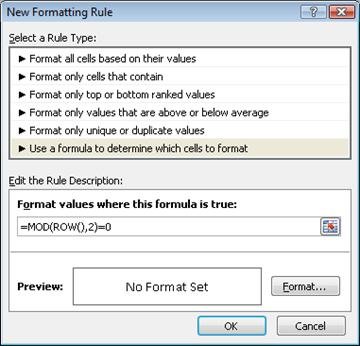
  3. Choose “New Rule.”
  4. Select “Use a formula to determine which cells to format.”
  5. Enter a formula based on your desired shading criteria (e.g., =MOD(ROW(),2)=0 for every other row).
  6. Click “Format” and choose the desired fill color.
  7. Click “OK” to apply the formatting.

2. Using the “Format as Table” Option:

• Steps:
  1. Select the range of cells you want to format as a table.
  2. Go to the “Home” tab and click “Format as Table.”
  3. Choose a table style that includes banded rows or columns.
  4. To customize the shading, go to the “Table Design” tab and adjust the “Banded Rows” or “Banded Columns” options.

3. Manual Formatting:

• Steps:
  1. Select the cells you want to shade.
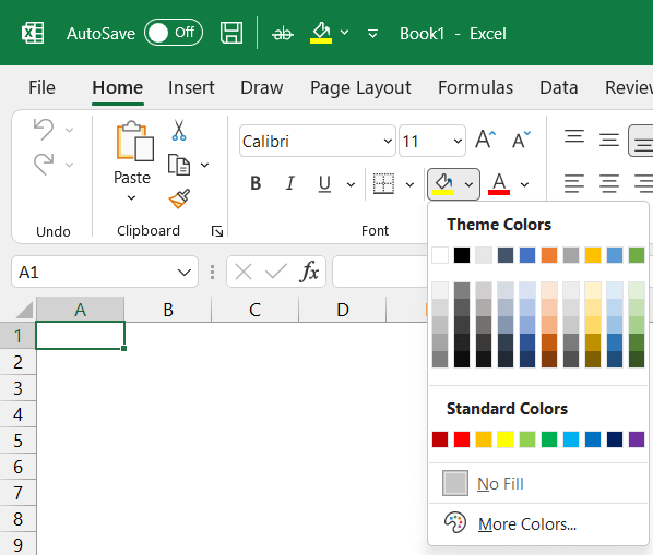
  2. Go to the “Home” tab and click the “Fill Color” button.
  3. Choose the desired color from the palette.

Tips for Effective Shading

• Choose Subtle Colors: Avoid using overly bright or distracting colors.
• Use a Consistent Pattern: Maintain a consistent shading pattern throughout your spreadsheet.
• Consider Accessibility: Ensure that the colors you choose are accessible to people with color vision deficiencies.
• Don’t Overdo It: Use shading sparingly to avoid overwhelming your spreadsheet.

Conclusion

Shading rows and columns in Excel is a simple yet powerful way to enhance the visual presentation of your data. By following the techniques outlined in this guide, you can create more organized, readable, and aesthetically pleasing spreadsheets. Whether you’re using conditional formatting, table styles, or manual formatting, a little bit of shading can go a long way in improving your Excel experience.

Related articles

» How to Delete Multiple Rows in Excel: A Quick and Easy Guide
» Transpose Excel columns to Rows in Excel chart
» How to Limit Rows and Columns in an Excel Worksheet